
As said previously, the third and final part of this series we shall use to have a look at the presentation of CFD simulation results offered by SOLIDWORKS Flow Simulation (abbreviated hereinafter as FS).
Part 1 of this series is dedicated to the set-up of this simulation.
Part 2 of this series is dedicated to the pre-solving and solving processes.
FS offers quite several ways to visualise as well as analyse numerically the results obtained from the solving process.
1. Mesh
The mesh option allows for the display of the mesh used in the calculation process. One may wish to view the meshing if the mesh has been generated automatically, or automatic refinement has been applied during the solving process (a feature we had not made use of in the previous episode when setting up the solver).
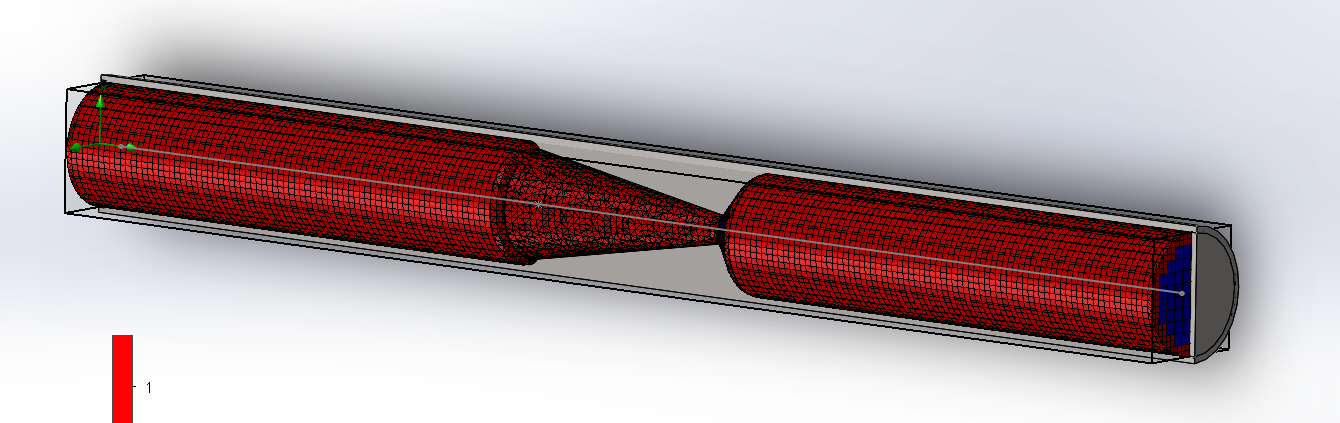
A display of the mesh of the model concerned will look like the following. Note that, because the meshing of FS is Cartesian, rather than body-fitted (as discussed in the beginning of episode 2, and we shall see later), the meshing has taken this specific form.
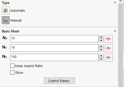
We can further explore the meshing of FS by examining the settings available for manual meshing. As we can see in the following screenshot, the fundamental meshing method of FS is dividing the computational domain in the XYZ directions into a number of cells respectively, and refine from there. We shall not go into further details here.
2. Cut plots
The cut plot function can be used to plot a number of quantities (their magnitude) against spacial position on an imaginary cut plane. The feature image of this series is a cut plot in the middle plane of the tube, plotting Mach number against position. Other ways of illustration, such as contours, flow vectors, streamlines, and cells, may be activated or deactivated, either singly or in combination, in one cut plot.
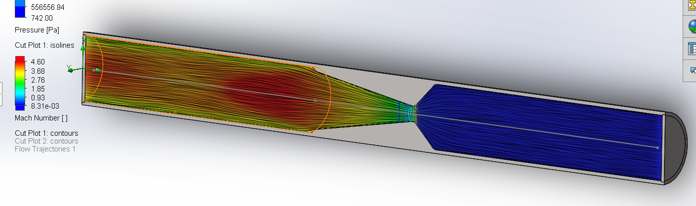
Below is a sample cut plot in the middle plane of the tube, plotting Mach number against spacial position, and with contours and streamlines shown. We can here visualise the rapid acceleration of the fluid across the narrowest part of the nozzle, by noting the rapid change in colour or a concentration of contours, denoting a steep gradient of the Mach number.
Cut plots can be useful for this kind of chambers where symmetry is present, or visualisation of the exterior is not available. A section is a convenient feature in analytical fluid mechanics, so cut plots make the same level of sense.
3. Surface plots
A surface plot has all the same features as a cut plot, other than the plot must be on a real surface of the solid model. This is useful for visualising the interaction of the fluid and the solid. For example, we might wish to visualise the pressure on the wall of the tube. Below is a surface plot of pressure against spacial position on all surfaces of the tube. A specific set of surfaces instead of all surfaces can be chosen, and features like contours, and vectors and streamlines, can be added to the plot.
It should be noted that, although the solid model is displayed in a cut-away view, the surface plot is cylindrical, which is the direct consequence of the fact that a surface plot must be on a surface of the solid model, which is round.
We can here visualise the dramatic drop of static pressure as the flow accelerate from almost stationary in the upstream section to supersonic speed downstream of the nozzle.
4. Isosurfaces
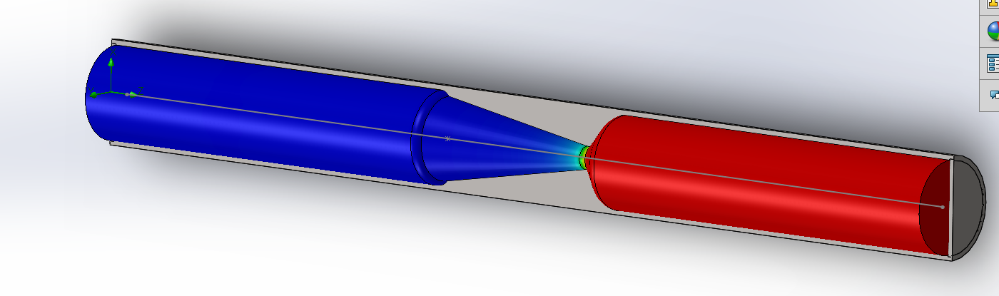
As the name suggest, this function allows for the plotting of iso-something surfaces within the computational domain. Commonly used are isobar surfaces and isothermal surfaces. In this case I shall plot a iso-Mach number surface around the supersonic nozzle. One-by-one definition of parameters or otherwise defined intervals are permitted in FS.
In the following image, the isosurfaces of 1 Mach, 2 Mach, and 3 Mach (an example of one-by-one definition), is plotted.
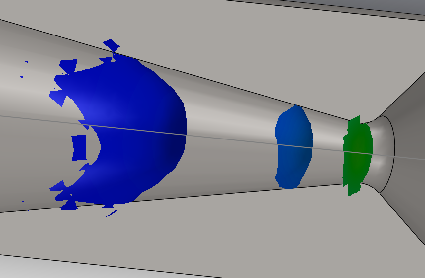
The green surface is the 1 Mach isosurface. We can realise that this is indeed at the position where the nozzle has the smallest cross-sectional area, as suggested by compressible fluid mechanics. The bowed surface in blue is the 3 Mach isosurface. It takes the bowed shape because of the existence of boundary layers. We can (roughly) visualise the shape of the boundary layers by these isosurfaces. We also note in passing that the 2 Mach isosurface is much less bowed than the 3 Mach one, and, again as suggested by fluid mechanics, the boundary layer grows thicker quite rapidly as the flow travels against pressure gradient, and might separate if the expansion half of the nozzle is not as shallow as the one we have modelled.
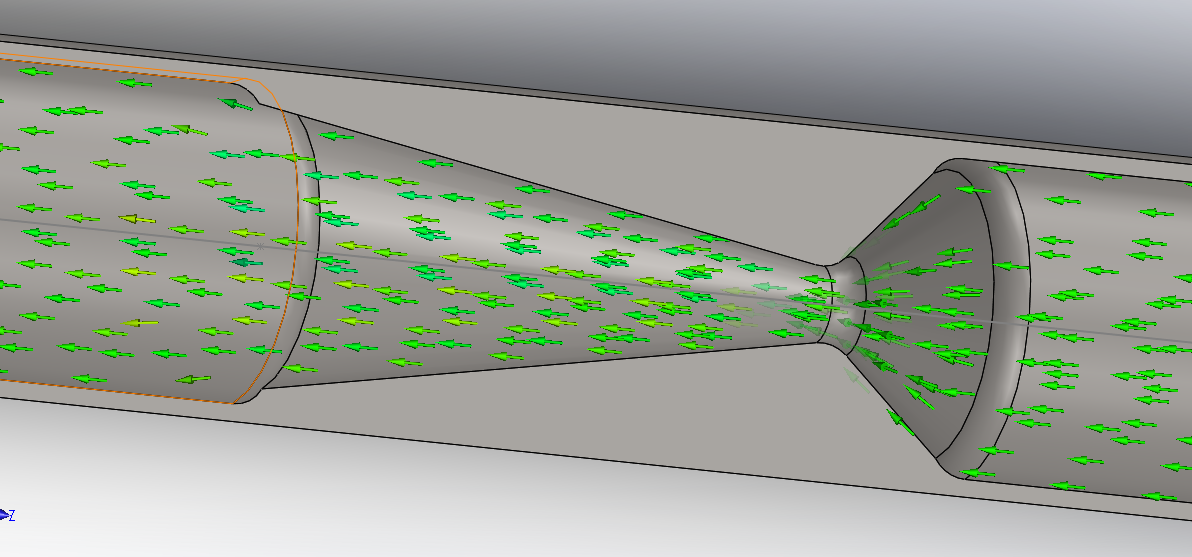
5. Flow trajectories
This function allows for the knowledge of “flow from where goes where”. In my opinion not a very useful feature for the analysis of the supersonic nozzle, but may be of importance in the study of a mixture device, for example.
The following sample is the trajectory of flow initiating from the upstream lid, and this is, indeed, where all the flow in this tube must come from. We note that radial velocity is negligible downstream of the throat of the nozzle as the axial velocity is huge. This can be seen by the direction where the arrows are pointing, comparing with the upstream contraction.
6. Particle studies
This feature allows the user to insert particles (solid or liquid) into the computational domain at given positions, at a given mass flow rate, and in a specified thermodynamic status, and study their subsequent motion under the influence of the flow field. Again not a particularly useful feature for the supersonic nozzle. It should be noted that, although the flow field has been solved for, the particle study requires additional computation, so it may not be instantly available. Other effects of particles, such as erosion of the solid model, is available.
7. Point, surface, and volume parameters
These belong to the numerical analytical functions available in the after-processing of FS, rather than the kind of visualising we have seen before. However, FS cannot do the numerical processing by itself, but instead it allows the user to define a point, a surface, or a volume, and specify the quantities of interest, and FS can then export the required data in .xlsx form to be analysed in Excel. This is much like what we have seen in the previous episodes, but what I have included there is a goal plot, as we shall see very soon. These are not interesting features so we shall not go into the details of their operation, but only touch on this possibility.
8. XY plots
A potentially very useful feature, and one of the advantages of integrating CFD with the solid modelling software package. The XY plots function allows for the plotting along a specified path, of a specified numerical quantity against either length of the path or XYZ coordinates for points on the path.
For this example, I am interested in the evolution of Mach number along the length of the axis of symmetry of the tube. I can first sketch a path along the axis of symmetry, effectively a straight line along the Z axis. Then I can make an XY plot of Mach number against length along the path. The final plot looks like follows:
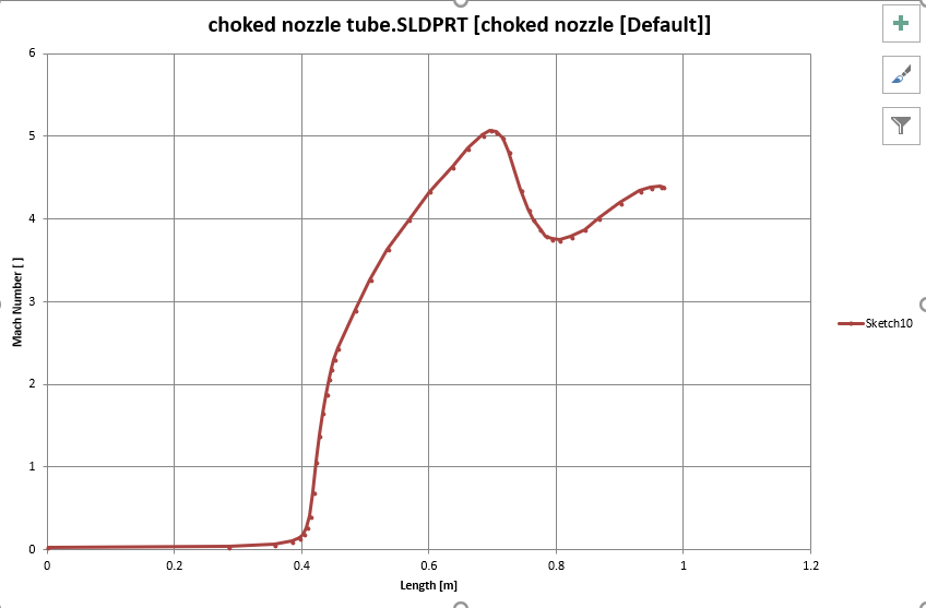
Note here that, because flow is flowing against Z direction, a flip of direction is required. Besides, this plot is generated in Excel rather than FS, because Excel is much more powerful in processing data than FS. FS allows for the export of plot data into Excel and we can manipulate such data as we wish.
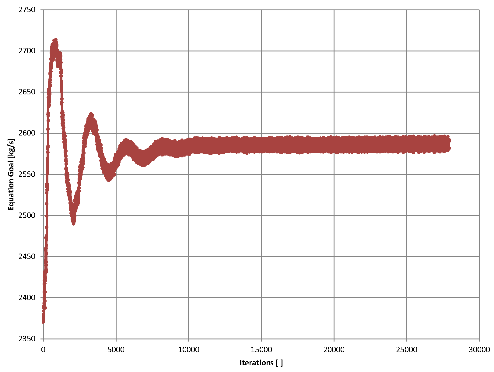
9. Goal plots
These we have seen in part 2 of this series. Because FS does a transient analysis by solving time-explicit Navier Stokes equations, these plots are really plots of values of the goals against time (or against iterations if one insist so, equivalently). The progress history towards steadiness (convergence, as discussed in part 2) is available for view, and, by generating such a plot in Excel, FS also exports all data for each iteration (there could be millions of them) into the Excel spreadsheet for analysis.
For a more detailed discussion, please see part 2 of this series.
Conclusion
FS offers a rather decent toolkit for the presentation and analysis of results. Visualisation of computational results is available in various forms. FS is not functional in the numerical processing of results, but one can conveniently export data of interest into Excel spreadsheets.
FS and SOLIDWORKS indeed are middle-of-the-way software packages, as their price and performance suggest. Nevertheless it is functional for small scaled projects, and it is very good at what it is capable of. I would recommend SOLIDWORKS and FS as a good starting point in the learning of design, solid modelling, and CFD.