
In the previous part we have illustrated and discussed the basic set up process for a SOLIDWORKS Flow Simulation CFD project. This part of the series is dedicated to the preparation of the solving process, and the actual solving process. It was originally planned that this series should be only of two posts’ length, however I have decided that the solving process must be elaborated as appropriate and, therefore, the result analysis part will be presented in part 3.
We have discussed that the solver’s stop conditions must be defined before the actual solving process could proceed. I believe it worthwhile to discuss the concept of convergence in this scenario. This comment from Bill McEachern I regard as worthwhile to quote in length:
FS runs the time averaged formulation of the Navier Stokes equations which means it essentially does a transient analysis (time explicit) solution so there is no real “converging” going on. Rather, for a (quasi) steady state solution (they don’t call it fluid dynamics for nothing) the program runs till the (typically) impulsive start-up has died out and it gets more or less “steady” (not varying much in time).
So I think your question is how does it know when this has happened? Well, if you do nothing it has preset termination criteria for given problem types – like 4 “travels” is the default. A travel is the number of iterations it takes for a disturbance to fully propagate across the domain. (Note here, in the solving process, there is a definitive number called “iterations per travel” presented by the solver. This implies that each iteration calculated by FS is a time explicit solution at a particular time, and the time increment across iterations is a certain division of a travel as determined by the solver)
Further, you can add goals and the program can use those and will stop when the goals you have assign stop changing. When you use goals (the recommended approach) you will be able to see the “convergence” trajectories (really they are time trajectories, as we shall see soon). When they flatten out and remain essentially invariant for some number of iterations (you can be the judge or you can let the program decide, again, as we shall see) then you can consider the particular result “achieved” or “converged”.
Given that FS is a “cart” code (cartesian) is suffers much reduced numerical diffusion issues compared to many body fitted codes (such as Fluent) and will typically “converge” for an incompressible flow problem in the order of low hundreds of iterations where as a similar problem in Fluent may require several thousand at very much higher cell counts – as a fluent guy once remarked “How does FS get the same answer as with 200,000 cells and 2 hours as Fluent with 2 million cells and 18 hours?” Then again FS doesn not have all the physics that Fluent supports but for what it does do it does a very fine job at it most of the time, at least in my experience.
From the discussion above, we can conclude that there are several basic ways to set the stop condition for the solver:
- default condition: calculate for a continuous period of 4 travels
- time limit: calculate for a certain number of travels (this is devised from the first automatic condition, and we can modify the travel amount as we like)
- calculation time limit: only calculate for a certain period of actual time (say, 1 hour), note the difference between 2 and 3
- iteration number limit: only calculate for a certain number of iterations (say, 2000)
- goal automatic convergence: set up a goal and specify that this goal would be used in convergence control (the default assumption if no action were taken is that convergence control is to be used), and the criteria for convergence is automatically determined by the solver
- goal manual convergence: set up a goal and specify that convergence control is to be used, and specify the convergence criteria by hand, e.g. specify a numerical value which the absolute variation of a result between the average and the extreme in an interval are not to exceed before convergence is to be declared, or a percentage similarly
- a combination of the above, note that logical operations are used between these conditions, namely OR and AND operations. In FS terms these are called “One Satisfied” and “All Satisfied” respectively.
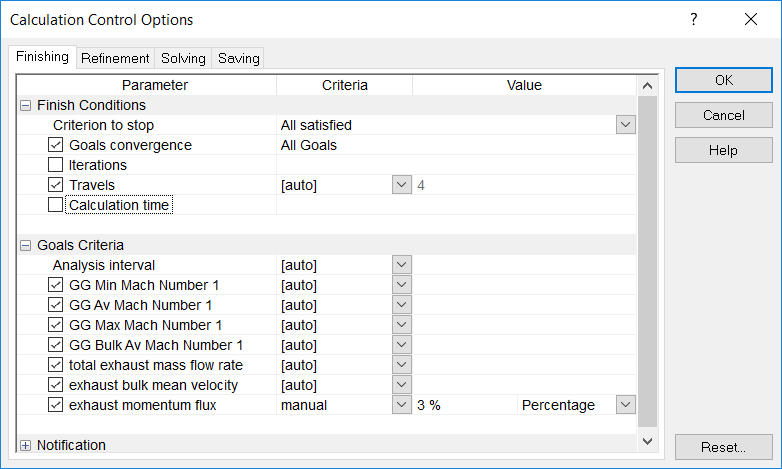
Presented above is an example of the control of the stop conditions, which is the one I have used for this project. Here, we have two criteria active, namely goal convergence of all goals, and 4 travels. These two are combined as a logical AND, as we shall see from the first row “all satisfied”. In the Goals Criteria section, all the goals are ticked, which means all of these are to be used in percentage control. The criteria for “convergence” are all set to AUTO except the last one, exhaust momentum flux (which is really the gross thrust of the propelling nozzle), convergence criterion of which I have manually set to 3%.
A note about the “analysis interval” option: in order to determine convergence, it is insufficient to look at the change between two iterations, or several iterations indeed. When the flow is highly unsteady, the difference between iterations may change from small values to large values and back quite dramatically. The FS algorithm to determine convergence is to compare the most extreme value of a goal with the average value of the same goal over a certain interval. FS evaluates this continuously. If we plot the time variance (to be strict, iteration variance) of a value of a goal, one can imagine holding a pair of limits spanning a narrow band of 3% width travelling along the curve as it grows (as the solver works out more iterations), and convergence is to be declared once the curve fits between your limit bars for the length it reaches. The longer the interval is, the more strict the convergence criterion and the longer the time required (potentially) to achieve this convergence. One can leave this to the solver to decide or to specify this manually.
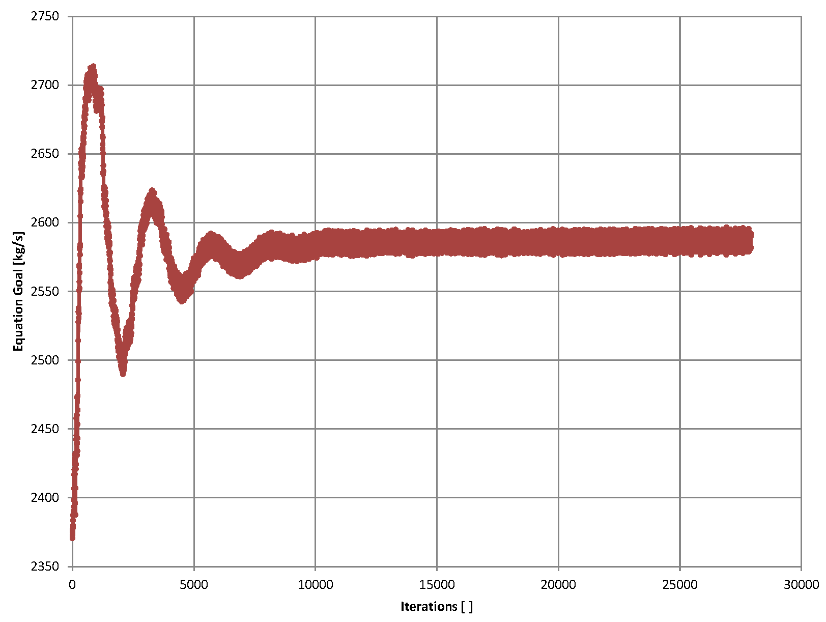
Please refer to the graph below, which plots the value of gross thrust against iterations. We have specified that this value must converge into a range of 3%. Although during solving process this is to be determined dynamically, we can do a bit of back analysis here. This value finally converged to around 2580, 3% of which should be 77.4. This goal actually converged at 4000 iterations, which is reasonable from our approximations above.
Another useful feature of the CFD is refinement. This allows the meshing to be refined during the solving process. We shall not make use of this feature in this project.
When all of these are defined, the solving can then proceed. One need to specify whether the solving is new or continued, whether this computer or a remote server is to be used, and how many cores of CPU to use, etc, which is out of the scope of our discussion.
Once solving has started, one must pay attention to the time taken to solve for 1 iteration, and the estimated time remaining presented by the solver. Occasionally very ambitious users try to solve for a very finely meshed model with complex flow on their laptops, only to find that it takes several minutes to solve for one iteration, and they have set a stop condition for a million iterations. It is critical to manage the processing power you have in hand when it is limited, and control the solving time to realistic intervals. One cannot do this without compromising on accuracy typically, but for serious CFD applications usually powerful servers are to be used, and the calculation can take several days if not weeks.
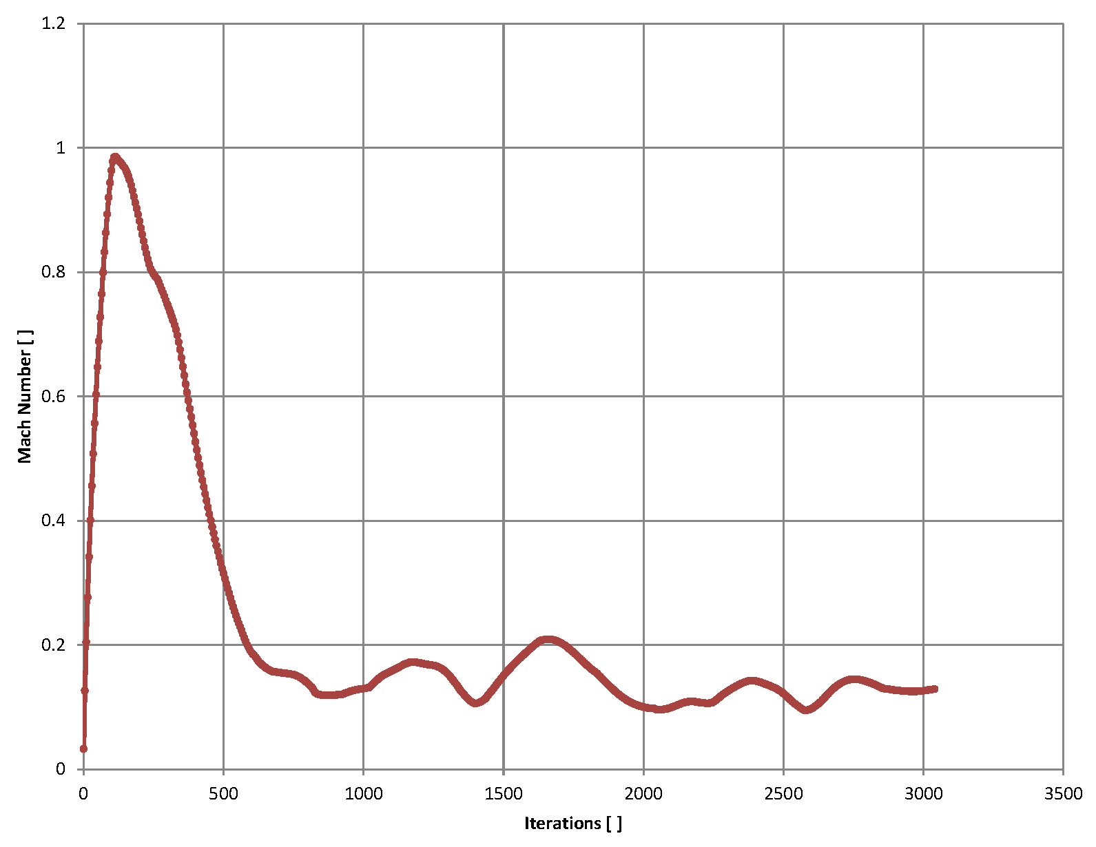
I consider it good practise to start with a very coarsely meshed model, say no more than 10000 cells for such a model I have constructed, and use loose convergence requirements, when a model is being solved for the first time. This can usually be done in a time of 10 minutes. This is not to produce meaningful results, but just to make sure that the model is being set up correctly. Occasionally one may find the goals they have set up is reading negative values, or high Mach number flow is detected where not expected, which may imply that the model is not watertight. These can be easily identified and corrected even with a coarse model, thereby saving much processing effort. One may also check that the goals they have set up is indeed converging, as we shall see in this plot: (this is a coarse check model for the project, 3500 iterations)
Only after you are satisfied that the model is correctly set up and the goals is indeed converging to a reasonable value that you would expect under the current scheme, should you refine the meshing and imply more strict convergence requirements, i.e. proceed with the actual solving process.
It is useful to monitor the solving process, which can easily take hours, and the effort pays off when something physically wrong is spotted (which can usually be done by a human). FS offers convenient GUI for users to do this.
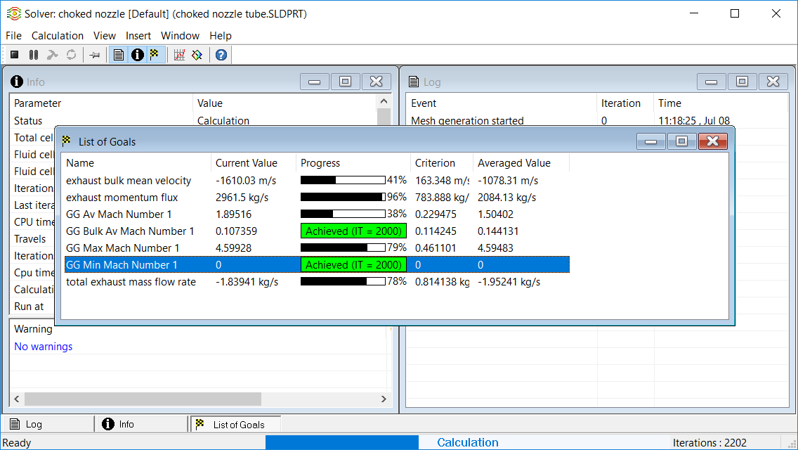
One can monitor the list of goals they have set up and watch they progress to convergence. Occasionally in the initial phase of a calculation the goals may seem diverging, i.e. the progress will actually roll backwards. Experienced users can identify whether this is just the transient response of the system since FS is really doing a time explicit analysis, or if the goal is not converging at all due to turbulent flow, due to too tight a convergence requirement, due to associated numerical error, or other physical reasons. An achieved goal may also cease to be convergent as time elapses. Human intervention would be useful under certain circumstances. However, if the initial check run is being done properly, there should be nothing seriously wrong with the set up of the model.
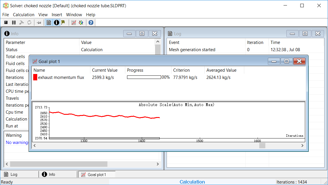
One can also graphically watch the value of a goal progress, as the following image illustrates.
Once the solver is finished, by default the results would be loaded automatically. FS saves its results in files which are, by default, in the same directory as the solid model file. If one decide to move those files, it is then necessary to re-establish the dependency by manually loading the file.
In the next part of the series, we shall discuss the presentation and processing of the results.